Real gas

Real gases – as opposed to a perfect or ideal gas – exhibit properties that cannot be explained entirely using the ideal gas law. To understand the behaviour of real gases, the following must be taken into account:

compressibility effects;
variable specific heat capacity;
van der Waals forces;
non-equilibrium thermodynamic effects;
issues with molecular dissociation and elementary reactions with variable composition.

For most applications, such a detailed analysis is unnecessary, and the ideal gas approximation can be used with reasonable accuracy. On the other hand, real-gas models have to be used near the condensation point of gases, near critical points, at very high pressures, to explain the Joule–Thomson effect and in other less usual cases.

Models

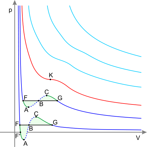
Isotherms of real gas(*) Dark blue curves – isotherms below the critical temperature. Green sections – metastable states.

The section to the left of point F – normal liquid.
Point F – boiling point.
Line FG – equilibrium of liquid and gaseous phases.
Section FA – superheated liquid.
Section F′A – stretched liquid (p<0).
Section AC – analytic continuation of isotherm, physically impossible.
Section CG – supercooled vapor.
Point G – dew point.
The plot to the right of point G – normal gas.
Areas FAB and GCB are equal.

Red curve – Critical isotherm.
Point K – critical point.

Light blue curves – supercritical isotherms

Main article: Equation of state
van der Waals model
Main article: van der Waals equation

Real gases are often modeled by taking into account their molar weight and molar volume

\( RT=\left(P+\frac{a}{V_\text{m}^2}\right)(V_\text{m}-b) \)

Where P is the pressure, T is the temperature, R the ideal gas constant, and V_m the molar volume. a and b are parameters that are determined empirically for each gas, but are sometimes estimated from their critical temperature (T_c) and critical pressure (P_c) using these relations:

\( a=\frac{27R^2T_\text{c}^2}{64P_\text{c}}\)

\( b=\frac{RT_\text{c}}{8P_\text{c}}\)

Redlich–Kwong model

The Redlich–Kwong equation is another two-parameter equation that is used to model real gases. It is almost always more accurate than the van der Waals equation, and often more accurate than some equations with more than two parameters. The equation is

\( RT=P(V_\text{m}-b)+\frac{a}{V_\text{m}(V_\text{m}+b)T^\frac{1}{2}}(V_\text{m}-b)

where a and b two empirical parameters that are not the same parameters as in the van der Waals equation. These parameters can be determined:

\( a=0.4275\frac{R^2T_\text{c}^{2.5}}{P_\text{c}}\)

\( b=0.0867\frac{RT_\text{c}}{P_\text{c}}\)

Berthelot and modified Berthelot model

The Berthelot equation (named after D. Berthelot[1] is very rarely used,

\( P=\frac{RT}{V_\text{m}-b}-\frac{a}{TV_\text{m}^2}\)

but the modified version is somewhat more accurate

\( P=\frac{RT}{V_\text{m}}\left[1+\frac{9P/P_\text{c}}{128T/T_\text{c}}\left(1-\frac{6}{(T/T_\text{c})^2}\right)\right]\)

Dieterici model

This model (named after C. Dieterici[2]) fell out of usage in recent years

\( P=RT\frac{\exp{(\frac{-a}{V_\text{m}RT})}}{V_\text{m}-b}.\)

Clausius model

The Clausius equation (named after Rudolf Clausius) is a very simple three-parameter equation used to model gases.

\( RT=\left(P+\frac{a}{T(V_\text{m}+c)^2}\right)(V_\text{m}-b)\)

where

\( a=\frac{27R^2T_\text{c}^3}{64P_\text{c}}\)

\( b=V_\text{c}-\frac{RT_\text{c}}{4P_\text{c}}\)

\( c=\frac{3RT_\text{c}}{8P_\text{c}}-V_\text{c}\)

where V_c is critical volume.

Virial model

The Virial equation derives from a perturbative treatment of statistical mechanics.

\( PV_\text{m}=RT\left(1+\frac{B(T)}{V_\text{m}}+\frac{C(T)}{V_\text{m}^2}+\frac{D(T)}{V_\text{m}^3}+...\right)

\)

or alternatively

\( PV_\text{m}=RT\left(1+\frac{B^\prime(T)}{P}+\frac{C^\prime(T)}{P^2}+\frac{D^\prime(T)}{P^3}+...\right)

\)

where A, B, C, A′, B′, and C′ are temperature dependent constants.

Peng–Robinson model

Peng–Robinson equation of state (named after D.-Y. Peng and D. B. Robinson[3]) has the interesting property being useful in modeling some liquids as well as real gases.

\( P=\frac{RT}{V_\text{m}-b}-\frac{a(T)}{V_\text{m}(V_\text{m}+b)+b(V_\text{m}-b)}\)

Wohl model

The Wohl equation (named after A. Wohl[4]) is formulated in terms of critical values, making it useful when real gas constants are not available.

\(RT=\left(P+\frac{a}{TV_\text{m}(V_\text{m}-b)}-\frac{c}{T^2V_\text{m}^3}\right)(V_\text{m}-b)\)

where

\(a=6P_\text{c}T_\text{c}V_\text{c}^2\)

\(b=\frac{V_\text{c}}{4}\)

\(c=4P_\text{c}T_\text{c}^2V_\text{c}^3.\)

Beattie–Bridgeman model

[5]

This equation is based on five experimentally determined constants. It is expressed as

\(P=\frac{RT}{v^2}\left(1-\frac{c}{vT^3}\right)(v+B)-\frac{A}{v^2}\)

where

\( A = A_0 \left(1 - \frac{a}{v} \right)\)
\( B = B_0 \left(1 - \frac{b}{v} \right)\)

This equation is known to be reasonably accurate for densities up to about 0.8 ρcr, where ρcr is the density of the substance at its critical point. The constants appearing in the above equation are available in following table when P is in KPa, v is in \( \frac{\text{m}^3}{\text{K}\,\text{mol}}\) , T is in K and \( \( R=8.314\frac{\text{kPa}\cdot\text{m}^3}{\text{K}\,\text{mol}\cdot\text{K}}\) [6]

Gas	A0	a	B0	b	c
Air	131.8441	0.01931	0.04611	-0.001101	4.34×10^4
Argon, Ar	130.7802	0.02328	0.03931	0.0	5.99×10^4
Carbon Dioxide, CO2	507.2836	0.07132	0.10476	0.07235	6.60×10^5
Helium, He	2.1886	0.05984	0.01400	0.0	40
Hydrogen, H2	20.0117	-0.00506	0.02096	-0.04359	504
Nitrogen, N2	136.2315	0.02617	0.05046	-0.00691	4.20×10^4
Oxygen, O2	151.0857	0.02562	0.04624	0.004208	4.80×10^4

Benedict–Webb–Rubin model
Main article: Benedict–Webb–Rubin equation

The BWR equation, sometimes referred to as the BWRS equation,

\( P=RTd+d^2\left(RT(B+bd)-(A+ad-a{\alpha}d^4)-\frac{1}{T^2}[C-cd(1+{\gamma}d^2)\exp(-{\gamma}d^2)]\right)\)

where d is the molar density and where a, b, c, A, B, C, α, and γ are empirical constants. Note that the γ constant is a derivative of constant α and therefore almost identical to 1.

See also

Gas laws
Ideal gas law by Boyle & Gay-Lussac
Compressibility factor
Equation of state

References

D. Berthelot in Travaux et Mémoires du Bureau international des Poids et Mesures – Tome XIII (Paris: Gauthier-Villars, 1907)
C. Dieterici, Ann. Phys. Chem. Wiedemanns Ann. 69, 685 (1899)
Peng, D. Y., and Robinson, D. B. (1976). "A New Two-Constant Equation of State". Industrial and Engineering Chemistry: Fundamentals 15: 59–64. doi:10.1021/i160057a011.
A. Wohl "Investigation of the condition equation", Zeitschrift für Physikalische Chemie (Leipzig) 87 pp. 1–39 (1914)
Yunus A. Cengel and Michael A. Boles, Thermodynamics: An Engineering Approach 7th Edition, McGraw-Hill, 2010, ISBN 007-352932-X

Gordan J. Van Wylen and Richard E. Sonntage, Fundamental of Classical Thermodynamics, 3rd ed, New York, John Wiley & Sons, 1986 P46 table 3.3

Dilip Kondepudi, Ilya Prigogine, Modern Thermodynamics, John Wiley & Sons, 1998, ISBN 0-471-97393-9
Hsieh, Jui Sheng, Engineering Thermodynamics, Prentice-Hall Inc., Englewood Cliffs, New Jersey 07632, 1993. ISBN 0-13-275702-8
Stanley M. Walas, Phase Equilibria in Chemical Engineering, Butterworth Publishers, 1985. ISBN 0-409-95162-5
M. Aznar, and A. Silva Telles, A Data Bank of Parameters for the Attractive Coefficient of the Peng–Robinson Equation of State, Braz. J. Chem. Eng. vol. 14 no. 1 São Paulo Mar. 1997, ISSN 0104-6632
An introduction to thermodynamics by Y. V. C. Rao
The corresponding-states principle and its practice: thermodynamic, transport and surface properties of fluids by Hong Wei Xiang

External links

http://www.ccl.net/cca/documents/dyoung/topics-orig/eq_state.html

Physics Encyclopedia