.

The Gram–Charlier A series (named in honor of Jørgen Pedersen Gram and Carl Charlier), and the Edgeworth series (named in honor of Francis Ysidro Edgeworth) are series that approximate a probability distribution in terms of its cumulants. The series are the same; but, the arrangement of terms (and thus the accuracy of truncating the series) differ.

Gram–Charlier A series

The key idea of these expansions is to write the characteristic function of the distribution whose probability density function is F to be approximated in terms of the characteristic function of a distribution with known and suitable properties, and to recover F through the inverse Fourier transform.

We examine a continuous random variable. Let f be the characteristic function of its distribution whose density function is F, and \( \kappa_r \) its cumulants. We expand in terms of a known distribution with probability density function Ψ, characteristic function ψ, and cumulants \( \gamma_r \) . The density Ψ is generally chosen to be that of the normal distribution, but other choices are possible as well. By the definition of the cumulants, we have the following formal identity:

\( f(t)=\exp\left[\sum_{r=1}^\infty(\kappa_r-\gamma_r)\frac{(it)^r}{r!}\right]\psi(t)\,. \)

By the properties of the Fourier transform, \( (it)^r\psi(t) is the Fourier transform of \( (-1)^r[D^r\Psi](-x) \) , where D is the differential operator with respect to x. Thus, after changing x with -x on both sides of the equation, we find for F the formal expansion

\( F(x) = \exp\left[\sum_{r=1}^\infty(\kappa_r - \gamma_r)\frac{(-D)^r}{r!}\right]\Psi(x)\,. \)

If Ψ is chosen as the normal density with mean and variance as given by F, that is, mean \( \mu = \kappa_1 \) and variance \( \sigma^2 = \kappa_2 \) , then the expansion becomes

\( F(x) = \exp\left[\sum_{r=3}^\infty\kappa_r\frac{(-D)^r}{r!}\right]\frac{1}{\sqrt{2\pi}\sigma}\exp\left[-\frac{(x-\mu)^2}{2\sigma^2}\right]. \)

By expanding the exponential and collecting terms according to the order of the derivatives, we arrive at the Gram–Charlier A series. If we include only the first two correction terms to the normal distribution, we obtain

\( F(x) \approx \frac{1}{\sqrt{2\pi}\sigma}\exp\left[-\frac{(x-\mu)^2}{2\sigma^2}\right]\left[1+\frac{\kappa_3}{3!\sigma^3}H_3\left(\frac{x-\mu}{\sigma}\right)+\frac{\kappa_4}{4!\sigma^4}H_4\left(\frac{x-\mu}{\sigma}\right)\right]\,, \)

with \( H_3(x)=x^3-3x \) and \( H_4(x)=x^4 - 6x^2 + 3 \) (these are Hermite polynomials).

Note that this expression is not guaranteed to be positive, and is therefore not a valid probability distribution. The Gram–Charlier A series diverges in many cases of interest—it converges only if F(x) falls off faster than \( \exp(-(x^2)/4) \) at infinity (Cramér 1957). When it does not converge, the series is also not a true asymptotic expansion, because it is not possible to estimate the error of the expansion. For this reason, the Edgeworth series (see next section) is generally preferred over the Gram–Charlier A series.

Edgeworth series

Edgeworth developed a similar expansion as an improvement to the central limit theorem. The advantage of the Edgeworth series is that the error is controlled, so that it is a true asymptotic expansion.

Let {Xi} be a sequence of independent and identically distributed random variables with mean μ and variance σ2, and let Yn be their standardized sums:

\( Y_n = \frac{1}{\sqrt{n}} \sum_{i=1}^n \frac{X_i - \mu}{\sigma}. \)

Let Fn denote the cumulative distribution functions of the variables Yn. Then by the central limit theorem,

\( \lim_{n\to\infty} F_n(x) = \Phi(x) \equiv \int_{-\infty}^x \tfrac{1}{\sqrt{2\pi}}e^{-\frac{1}{2}q^2}dq \)

for every x, as long as the mean and variance are finite.

Now assume that the random variables Xi have mean μ, variance σ2, and higher cumulants κr=σrλr. If we expand in terms of the standard normal distribution, that is, if we set

\( \Psi(x)=\frac{1}{\sqrt{2\pi}}\exp(-\tfrac{1}{2}x^2) \)

then the cumulant differences in the formal expression of the characteristic function fn(t) of Fn are

\( \kappa^{F(n)}_1-\gamma_1 = 0, \)
\( \kappa^{F(n)}_2-\gamma_2 = 0, \)
\( \kappa^{F(n)}_r-\gamma_r = \frac{\kappa_r}{\sigma^rn^{r/2-1}} = \frac{\lambda_r}{n^{r/2-1}}; \qquad r\geq 3. \)

The Edgeworth series is developed similarly to the Gram–Charlier A series, only that now terms are collected according to powers of n. Thus, we have

\( f_n(t)=\left[1+\sum_{j=1}^\infty \frac{P_j(it)}{n^{j/2}}\right] \exp(-t^2/2)\,, \)

where Pj(x) is a polynomial of degree 3j. Again, after inverse Fourier transform, the density function Fn follows as

\( F_n(x) = \Phi(x) + \sum_{j=1}^\infty \frac{P_j(-D)}{n^{j/2}} \Phi(x)\,. \)

The first five terms of the expansion are[1]

\( \begin{align} F_n(x) &= \Phi(x) \\ &\quad -\frac{1}{n^{\frac{1}{2}}}\left(\tfrac{1}{6}\lambda_3\,\Phi^{(3)}(x) \right) \\ &\quad +\frac{1}{n}\left(\tfrac{1}{24}\lambda_4\,\Phi^{(4)}(x) + \tfrac{1}{72}\lambda_3^2\,\Phi^{(6)}(x) \right) \\ &\quad -\frac{1}{n^{\frac{3}{2}}}\left(\tfrac{1}{120}\lambda_5\,\Phi^{(5)}(x) + \tfrac{1}{144}\lambda_3\lambda_4\,\Phi^{(7)}(x) + \tfrac{1}{1296}\lambda_3^3\,\Phi^{(9)}(x)\right) \\ &\quad + \frac{1}{n^2}\left(\tfrac{1}{720}\lambda_6\,\Phi^{(6)}(x) + \left(\tfrac{1}{1152}\lambda_4^2 + \tfrac{1}{720}\lambda_3\lambda_5\right)\Phi^{(8)}(x) + \tfrac{1}{1728}\lambda_3^2\lambda_4\,\Phi^{(10)}(x) + \tfrac{1}{31104}\lambda_3^4\,\Phi^{(12)}(x) \right)\\ &\quad + O \left (n^{-\frac{5}{2}} \right ). \end{align} \)

Here, Φ^(j)(x) is the j-th derivative of Φ(·) at point x. Remembering that the derivatives of the density of the normal distribution are related to the normal density by ϕ⁽ⁿ⁾(x) is (-1)ⁿH_n(x)ϕ(x), (where H_n is the Hermite polynomial of order n), this explains the alternative representations in terms of the density function. Blinnikov and Moessner (1998) have given a simple algorithm to calculate higher-order terms of the expansion.

Note that in case of a lattice distributions (which have discrete values), the Edgeworth expansion must be adjusted to account for the discontinuous jumps between lattice points.^[2]

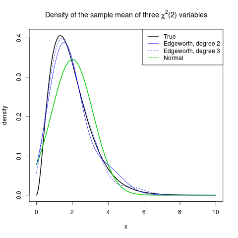
Illustration: density of the sample mean of 3 Χ²
Density of the sample mean of three chi2 variables. The chart compares the true density, the normal approximation, and two edgeworth expansions (*)

Take \( X_i \sim \chi^2(k=2) \qquad i=1, 2, 3 \) and the sample mean \( \bar X = \frac{1}{3} \sum_{i=1}^{3} X_i . \)

We can use several distributions for \(\bar X \) :

The exact distribution, which follows a gamma distribution: \( \bar X \sim \mathrm{Gamma}\left(\alpha=n\cdot k /2, \theta= 2/n \right) = \mathrm{Gamma}\left(\alpha=3, \theta= 2/3 \right) \)
The asymptotic normal distribution: \( \bar X \xrightarrow{n \to \infty} N(k, 2\cdot k /n ) = N(2, 4/3 ) \)
Two Edgeworth expansion, of degree 2 and 3

Disadvantages of the Edgeworth expansion

Edgeworth expansions can suffer from a few issues:

They are not guaranteed to be a proper probability distribution as:
The integral of the density needs not integrate to 1
Probabilities can be negative
They can be inaccurate, especially in the tails, due to mainly two reasons:
They are obtained under a Taylor series around the mean
They guarantee (asymptotically) an absolute error, not a relative one. This is an issue when one wants to approximate very small quantities, for which the absolute error might be small, but the relative error important.

References

Weisstein, Eric W., "Edgeworth Series", MathWorld.
Kolassa, John E.; McCullagh, Peter (1990). "Edgeworth series for lattice distributions". Annals of Statistics 18 (2): 981–985. JSTOR 2242145.
Further reading
H. Cramér. (1957). Mathematical Methods of Statistics. Princeton University Press, Princeton.
D. L. Wallace. (1958). "Asymptotic approximations to distributions". Annals of Mathematical Statistics, 29: 635–654.
M. Kendall & A. Stuart. (1977), The advanced theory of statistics, Vol 1: Distribution theory, 4th Edition, Macmillan, New York.
P. McCullagh (1987). Tensor Methods in Statistics. Chapman and Hall, London.
D. R. Cox and O. E. Barndorff-Nielsen (1989). Asymptotic Techniques for Use in Statistics. Chapman and Hall, London.
P. Hall (1992). The Bootstrap and Edgeworth Expansion. Springer, New York.
Hazewinkel, Michiel, ed. (2001), "Edgeworth series", Encyclopedia of Mathematics, Springer, ISBN 978-1-55608-010-4
S. Blinnikov and R. Moessner (1998). Expansions for nearly Gaussian distributions. Astronomy and astrophysics Supplement series, 130: 193–205.
J. E. Kolassa (2006). Series Approximation Methods in Statistics (3rd ed.). (Lecture Notes in Statistics #88). Springer, New York.
Undergraduate Texts in Mathematics
Graduate Studies in Mathematics
Retrieved from "http://en.wikipedia.org/"
All text is available under the terms of the GNU Free Documentation License