Bairstow's method

In numerical analysis, Bairstow's method is an efficient algorithm for finding the roots of a real polynomial of arbitrary degree. The algorithm first appeared in the appendix of the 1920 book "Applied Aerodynamics" by Leonard Bairstow. The algorithm finds the roots in complex conjugate pairs using only real arithmetic.

See root-finding algorithm for other algorithms.

Description of the method

Bairstow's approach is to use Newton's method to adjust the coefficients u and v in the quadratic \( x^2 + ux + v \) until its roots are also roots of the polynomial being solved. The roots of the quadratic may then be determined, and the polynomial may be divided by the quadratic to eliminate those roots. This process is then iterated until the polynomial becomes quadratic or linear, and all the roots have been determined.

Long division of the polynomial to be solved

\( P(x)=\sum_{i=0}^n a_i x^i \)

by x^2 + ux + v yields a quotient \( Q(x)=\sum_{i=0}^{n-2} b_i x^i and a remainder cx+d such that

\( P(x)=(x^2+ux+v)\left(\sum_{i=0}^{n-2} b_i x^i\right) + (cx+d).

A second division of Q(x) by x^2 + ux + v is performed to yield a quotient \( R(x)=\sum_{i=0}^{n-4} f_i x^i \) and remainder gx+h with

\( Q(x)=(x^2+ux+v)\left(\sum_{i=0}^{n-4} f_i x^i\right) + (gx+h). \)

The variables \(c,\,d,\,g,\,h, and the \(\{b_i\},\;\{f_i\} are functions of u and v. They can be found recursively as follows.

\( \begin{align} b_n &= b_{n-1} = 0,& f_n &= f_{n-1} = 0,\\ b_i &= a_{i+2}-ub_{i+1}-vb_{i+2}&f_i &= b_{i+2}-uf_{i+1}-vf_{i+2} \qquad (i=n-2,\ldots,0),\\ c &= a_1-ub_0-vb_1,& g &= b_1-uf_0-vf_1,\\ d & =a_0-vb_0,& h & =b_0-vf_0. \end{align} \)

The quadratic evenly divides the polynomial when

\( c(u,v)=d(u,v)=0. \, \)

Values of u and v for which this occurs can be discovered by picking starting values and iterating Newton's method in two dimensions

\( \begin{bmatrix}u\\ v\end{bmatrix} := \begin{bmatrix}u\\ v\end{bmatrix} - \begin{bmatrix} \frac{\partial c}{\partial u}&\frac{\partial c}{\partial v}\\[3pt] \frac{\partial d}{\partial u} &\frac{\partial d}{\partial v} \end{bmatrix}^{-1} \begin{bmatrix}c\\ d\end{bmatrix} := \begin{bmatrix}u\\ v\end{bmatrix} - \frac{1}{vg^2+h(h-ug)} \begin{bmatrix} -h & g\\[3pt] -gv & gu-h \end{bmatrix} \begin{bmatrix}c\\ d\end{bmatrix} \)

until convergence occurs. This method to find the zeroes of polynomials can thus be easily implemented with a programming language or even a spreadsheet.
Example

The task is to determine a pair of roots of the polynomial

\( f(x) = 6 \, x^5 + 11 \, x^4 - 33 \, x^3 - 33 \, x^2 + 11 \, x + 6. \)

As first quadratic polynomial one may choose the normalized polynomial formed from the leading three coefficients of f(x),

\( u = \frac{a_{n-1}}{a_n} = \frac{11}{6} ; \quad v = \frac{a_{n-2}}{a_n} = - \frac{33}{6}.\, \)

The iteration then produces the table

Nr	u	v	step length	roots
0	1.833333333333	-5.500000000000	5.579008780071	-0.916666666667±2.517990821623
1	2.979026068546	-0.039896784438	2.048558558641	-1.489513034273±1.502845921479
2	3.635306053091	1.900693009946	1.799922838287	-1.817653026545±1.184554563945
3	3.064938039761	0.193530875538	1.256481376254	-1.532469019881±1.467968126819
4	3.461834191232	1.385679731101	0.428931413521	-1.730917095616±1.269013105052
5	3.326244386565	0.978742927192	0.022431883898	-1.663122193282±1.336874153612
6	3.333340909351	1.000022701147	0.000023931927	-1.666670454676±1.333329555414
7	3.333333333340	1.000000000020	0.000000000021	-1.666666666670±1.333333333330
8	3.333333333333	1.000000000000	0.000000000000	-1.666666666667±1.333333333333

After eight iterations the method produced a quadratic factor that contains the roots -1/3 and -3 within the represented precision. The step length from the fourth iteration on demonstrates the superlinear speed of convergence.

\( f(x)=x^5-1\)

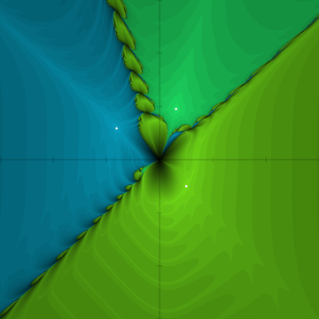
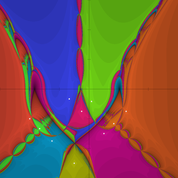
\( f(x)=x^6-x \)

\( \begin{align}f(x)=&6x^5+11x^4-33x^3\\&-33x^2+11x+6\end{align} \)

Performance

Bairstow's algorithm inherits the local quadratic convergence of Newton's method, except in the case of quadratic factors of multiplicity higher than 1, when convergence to that factor is linear. A particular kind of instability is observed when the polynomial has odd degree and only one real root. Quadratic factors that have a small value at this real root tend to diverge to infinity.

The images represent pairs \((s,t)\in[-3,3]^2 \) . Points in the upper half plane t>0 correspond to a linear factor with roots s\pm it, that is \( x^2+ux+v=(x-s)^2+t^2. \) Points in the lower half plane t<0 correspond to quadratic factors with roots s\pm t, that is, \(x^2+ux+v=(x-s)^2-t^2 \) , so in general \( (u,\,v)=(-2s,\, s^2+t\,|t|) \) . Points are colored according to the final point of the Bairstow iteration, black points indicate divergent behavior.

The first image is a demonstration of the single real root case. The second indicates that one can remedy the divergent behavior by introducing an additional real root, at the cost of slowing down the speed of convergence. One can also in the case of odd degree polynomials first find a real root using Newton's method and/or an interval shrinking method, so that after deflation a better-behaved even-degree polynomial remains. The third image corresponds to the example above.
External links

Bairstow's Algorithm on Mathworld
Numerical Recipes in Fortran 77 Online
Example polynomial root solver (deg(P)<=10) using Bairstow's Method
LinBairstowSolve, an open-source C++ implementation of the Lin-Bairstow method available as a method of the VTK library
Online root finding of a polynomial-Bairstow's method by Farhad Mazlumi

Mathematics Encyclopedia